R is an open source software application for data science. It’s a powerful language and has a ton of packages that streamline everything from performing operations on data sets to running machine learning algorithms.
Anyone in an “analyst” role in business that heavily uses Excel for data analysis should learn and use R. Excel is great for building pro-forma financial statements, but data analysis should be done in a statistical package such as R.
In this tutorial I’ll give you a 20 minute intro to R, doing the following:
- Importing two CSV (comma-separated value) files
- Investigating the structure and content of the data
- Merging the two CSV files
- Looking up a value in the merged file
You’ll need the following:
- R – the open source statistical programming package (download here: https://cran.cnr.berkeley.edu/)
- RStudio – a fantastic user interface for R that makes using R for data science much easier (download the Open Source Destktop version here: https://www.rstudio.com/products/rstudio/#Desktop)
- Sean Lahman’s Baseball Database – a set of historical baseball datasets (download the 2015 — comma-delimited version here: http://www.seanlahman.com/baseball-archive/statistics/)
I strongly encourage you to actually do the work along with me. The best way to learn programs such as R is to play around with them.
(Also, as a side note, another benefit of popular, open source programs like R is the huge community around them that are willing to help one another. If you ever need help doing something in R, you can easily find an answer by searching google and checking for answers on r-bloggers.com and stackexchange.com or by looking through the excellent documentation https://www.r-project.org/other-docs.html.)
Ok, go ahead and download and install R and RStudio on your computer then download the baseball database and store it in your Documents folder.
Step 1 – Create an RStudio Project
Create a folder called “Baseball” inside your “Documents” folder. Extract the baseball database zip file into the “Baseball” folder and you should now have a sub-folder called “baseballdatabank-master” within “Baseball”. Next, create a new folder called “R Baseball Project” inside of “Baseball”. So the folder “Baseball” should have two folders in it.
If you were to open “baseballdatabank-master” you would see a README file and another folder called “core” which contains all the CSV files. Each CSV contains a different dataset which can be merged using common fields.
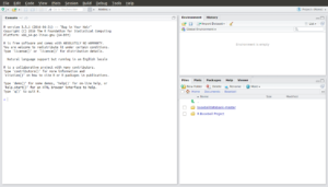
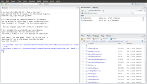
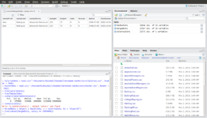
Now, open RStudio. You should see a screen that looks like this, though the actual files you see in the window on the bottom right might differ from mine.
Click on “File” (top left) then “New Project” then “Existing Directory” and browse to and select the “R Baseball Project” folder you created.
Congratulations, you’ve created your first RStudio project!
Step 2 – Use RStudio interface to look at a CSV file
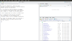
Looking back at the RStudio interface, you should see a window on the bottom right with a list of files in it. Above that window is a picture of a house and a directory navigation bar. On the screen shot for my system above it shows Home>Documents>Baseball. You can use that menu and the clickable folders in the window below it to navigate your computer and access files. Use that menu to navigate to the “Documents” folder.
You should then see a list of files and folders in the window below. Click on the “Baseball” folder and then on “baseballdatabase-master” then on “core”. Now you should see a list of all the CSV files in the window:
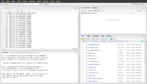
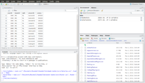
Now click on “Salaries.csv” (you’ll likely have to scroll down since the files should be sorted alphabetically). Notice that the file opens in a window in the top left of the screen and shows the CSV data just as we’d expect it to look:
Great. Now close the CSV file by clicking on the “x”. Congratulations, you’ve just used RStudio to view a raw data file in CSV format.
Step 3 – Import CSV files
Ok, now look at the column on the left half of the screen that says “Console”. This is the interactive console that R provides so we can issue commands. Let’s use the console to import the Salaries.csv file. Click your mouse after the “>” at the bottom of the console and type:
> SalariesData = read.csv(“~/Documents/Baseball/baseballdatabank-master/core/Salaries.csv”, header = TRUE)
(Warning: the correct start of the file path: “~/Documents/” varies depending on your operating system. “~/Documents/” should work for Linux or Mac while “C:\Users\your-username\Documents\” should work for Windows.)
Now hit “Enter” on the keyboard.
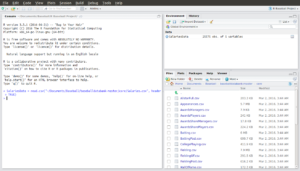
Notice how in the top right window, called “Data”, there is now a file called “SalariesData”:
So what happened here? Very simply, we told R that we wanted it to create something called “SalariesData” and to use the output from a function called read.csv to do it. The function read.csv is a function that exists in R specifically to help import CSV files.
The general format for a function in R is this: a function name (i.e. read.csv) followed by parentheses. The stuff inside the parentheses are parameters we pass to the function. In the case of the function read.csv(), two parameters we passed were the location of the CSV file and something telling R that the first row of the CSV contains the variable names (this is called a “header”) while the rest of the rows contain data.
R functions can have required parameters (in this case, the location of the CSV file is required) and optional parameters (we actually didn’t have to explicitly tell R that the first line of the file is a header as that assumption is built in to read.csv by default).
Functions are very common in R and there are much simpler examples. One such example is sqrt(). Unsurprisingly this is the function to calculate a square root. The parameter you pass is the number you want to calculate the square root of. So for example, if you type in the console:
> sqrt(9)
R will print “3” on the next line.
Ok, now let’s import the “Master.csv” file. Here’s the command:
> MasterData = read.csv(“~/Documents/Baseball/baseballdatabank-master/core/Master.csv”, header = TRUE)
And here’s the output:
Congratulations, you’ve just imported your first CSV files into R!
Step 4 – Investigate structure and content of the data
Now look at the objects in the “Data” window on the top right. These are R Data Frames, which are basically tables containing the data from the CSV files. In each data frame, the rows correspond to records and the columns to variables. Click on the blue arrow to the left of the SalariesData data frame. You can now see a list of all the variables in that data frame and then some information about the content of each variable (don’t worry about the content for now). Now click on the blue arrow again to close the details.
Now click on the name SalariesData and you should see a window open on the top left showing the data as a table:
Good, now click the “x” to close the table. Look at the console on the bottom left. Notice that the command “View(SalariesData)” shows up even though we didn’t type it. When we clicked on the data frame name to open it, RStudio issued the command for us. We could have also opened the data frame by typing that command into the console ourselves.
Now open the MasterData data frame. You can see that this data frame shows information about each player including his first and last name. We want to calculate which player had the highest salary in a single year, but SalariesData doesn’t have a variable showing player name. Instead it has a unique identifier for each player called playerID. The player names are in the MasterData file, which also has the field playerID. We will have to use that common field (playerID) to merge the two files so our output shows the actual player’s name.
Ok, close MasterData.
Go back to the console and type:
> summary(SalariesData$salary)
Your screen should look like this:
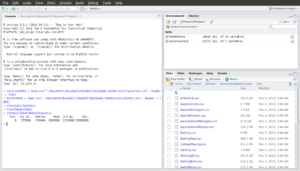
Ok, so what happened here? We used the summary() function to get R to show us quartiles for the salary data. The parameter we passed to summary() was the variable we wanted to see the quartiles for. The syntax here: SalariesData$salary is common in R. The text before the $ is the name of the data frame and the text after the $ is the variable. Telling R that we want a summary of the salary data – i.e. summary(salary) – isn’t sufficient, we also need to tell R which data frame has the salary data. Look at the error message we get if we forget to specify a data frame:
Ok, so a couple interesting things from the summary data: If you look at the salaries data again, you’ll see that it’s stated by player by year. So each record in that data is an observation for an individual player for a given year. So, we know from the summary() output that the highest salary ever paid to a player for a single year was $33,000,000 and that there is at least one player that was paid $0 for a year (or there is some error in the data).
Step 5 – Merge the data
Ok, now go to the console and type the command:
> MergedData = merge(x = MasterData, y = SalariesData, by = “playerID”)
Here we are creating a new data frame called MergedData by calling the function merge(). We are passing to merge() a few parameters, namely that the first data frame is MasterData (x = MasterData) and the second data frame is SalariesData (y = SalariesData). We are also passing a parameter to tell the function which field is common between the data frames, namely “playerID”.
Click on MergedData to open it:

Scroll over to the right in the view of MergedData and you’ll be able to see that it includes both the salaries data and the player names. Now, it’s important to never just trust that we’ll get the output we want when we’re doing data analysis. Notice that SalariesData has more observations than MasterData. Ok, we’d expect that as MasterData is just a roster of players while SalariesData shows player salaries over time hence many players will have multiple observations in SalariesData.
But look again at the number of observations for MergedData in the top right window. We might have expected that merging the data would just append the player names and other fields from MasterData to every observation in SalariesData. But MergedData has fewer observations than SalariesData, so we lost some records during the merge. This is because we called the merge() function without passing it any parameter to say what to do for any instances where there is a given playerID in one data frame but not in the other data frame. The default if we don’t pass merge() any parameters about how to handle those cases is for R to just exclude those observations from the merged data frame.
Step 6 – Find the player with the highest annual salary
Ok, so we now have a data frame with the annual salary data for each player merged with the players’ names (in addition to other data like height and weight). So, now let’s figure out who has the highest ever annual salary. We already know from running the summary() function earlier that the highest salary is $33,000,000, so all we have to do is find the record in MergedData that has an observation of 33000000 for “salary”. We can do this by subsetting the data with a function called subset() and keeping only the observation(s) where salary = 33000000. Run this code in the console:
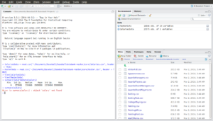
> View(subset(MergedData, salary == 33000000))
Here’s the output:
We can see that the player with the highest ever annual salary is Alex Rodriguez and that he earned that salary in both 2009 and 2010.
Now, View(subset(MergedData, salary == 33000000)) appears to be the most complicated code we’ve used so far. But we know how to think through what it’s doing. First, we are calling a function called subset() and we are passing it both a data frame (MergedData) that we want to pull a subset from and a condition (salary == 33000000). With this, subset() will return another data frame that is a subset of MergedData but only retaining rows where the salary observation is 33000000. Two things to note:
- We use a double equals sign (==) in R when we want to test a conditional statement. The single equals sign is used for giving a value to a variable (or to another object like a data frame).
- We can use “salary” instead of “MergedData$salary” because we are passing the function the data frame that it should use, so it’s redundant to also use MergedData$salary (though R would also accept it in this format and produce the same output).
We are then taking the data frame that subset() returned and passing it to the function View() which just displays the data in table format for us, just like when we clicked on the data frames in the “Data” window on the top right of the screen.
Notice that writing the function like this didn’t produce any new objects in the “Data” window. In prior work with data frames, we wrote, for example: “MergedData = merge(…)”. This syntax tells R to create a new object and set it equal to the output of the function (in this case, MergedData was the new object). By contrast, in the syntax View(subset(…)) we aren’t telling R to create any new objects for us. So we can get R to just run the operation and show us the result without saving a new data frame. If we wanted a new data frame saved showing just the observations for Alex Rodriguez in 2009 and 2010, we could have done:
> HighestSalary = subset(MergedData, salary == 33000000)
and then viewed it with:
> View(HighestSalary).
You may have noticed that we did something inefficient in this analysis. We merged the full Salaries data frame with the Master data frame before subsetting it to find the player with the highest salary. In subsetting, we discarded almost all of the Salaries data, so in effect we discarded almost all of the computing work we did to merge the two data sets. It would have been much more efficient to subset the data first and then perform the merge. For this tutorial we accepted the inefficiency for the purpose of illustrating how the merge function works. When doing data analysis for real, it’s important to think about how to do it efficiently, especially when working with large scale data or procedures that are repeated over and over.
Congratulations! If you’ve gone through all these steps, you have a very solid introduction to R. You know how to set up a project in RStudio, inspect raw CSV files, import CSV data into R data frames, look at summary statistics on a data frame, merge two data frames, and subset a data frame based on conditional criteria.
One additional thing to note about RStudio is that when you close it down (File → Quit Session), you will be asked if you want to save your workspace image to the R Project you created. If you want to work on this data again, click SAVE! The next time you want to work on the analysis, navigate to the folder where you saved your R Project (~/Documents/Baseball/R Baseball Project) and double click on R Baseball Project.Rproj. This will open your R project with all the data frames (and any other objects) you’ve created still intact.
Continue to our next tutorial: Get Started with AWS in 20 Minutes.